There are a few more essential skills that we need in our toolbox. In this
chapter, we will explore some of the powerful methods of kinematic trajectory
motion planning.
I'm actually almost proud of making it this far into the notes without
covering this topic yet. Writing a relatively simple script for the pose of
the gripper, like we did in the bin picking chapter, really can solve a lot of
interesting problems. But there are a number of reasons that we might want a
more automated solution:
When the environment becomes more cluttered, it is harder to write
such a simple solution, and we might have to worry about collisions between
the arm and the environment as well as the gripper and the environment.
If we are doing "mobile manipulation" -- our robotic arms are attached to
a mobile base -- then the robot might have to operate in many different environments. Even if the workspace is not geometrically complicated,
it might still be different enough each time we reach that it requires
automated (but possibly still simple) planning.
If the robot is
operating in a simple known environment all day long, then it probably makes
sense to optimize the trajectories that it is executing; we can often speed up
the manipulation process significantly.
In fact, if you ran the clutter
clearing demo, I would say that motion planning failures were the biggest
limitation of that solution so far: the hand or objects could sometimes
collide with the cameras or bins, or the differential-inverse kinematics
strategy (which effectively ignored the joint angles) would sometime cause the
robot to fold in on itself. In this chapter we'll develop the tools to
make that much better!
I do need to make one important caveat. For motion planning in
manipulation, lots of emphasis is placed on the problem of avoiding
collisions. Despite having done some work in this field myself, I actually
really dislike the problem formulation of collision-free motion planning. I
think that on the whole, robots are too afraid of bumping into the world
(because things still go wrong when they do). I don't think humans are
solving these complex geometric problems every time we reach... even when we
are reaching in dense clutter. I actually suspect that we are very bad at
solving them. I would much rather see robots that perform well even with very
coarse / approximate plans for moving through a cluttered environment, that
are not afraid to make incidental contacts, and that can still accomplish the
task when they do!
Inverse Kinematics
The goal of this chapter is to solve for motion trajectories. But I would argue that if you really understand how to solve inverse kinematics, then you've got most of what you need to plan trajectories.
We know that the forward kinematics
give us a (nonlinear) mapping from joint angles to e.g. the pose of the
gripper: $X^G = f_{kin}(q)$. So, naturally, one would think that the
problem of inverse kinematics (IK) is about solving for the inverse map, $q
= f^{-1}_{kin}(X^G).$ But, like we did with differential inverse
kinematics, I'd like to think about inverse kinematics as the more general
problem of finding joint angles subject to a rich library of costs and
constraints; and the space of possible kinematic constraints is indeed
rich.
For example, when we were evaluating grasp candidates for bin
picking, we had only a soft preference on the orientation of the hand
relative to some antipodal grasp. In that case, specifying 6 DOF pose of
the gripper and finding one set of joint angles which satisfies it exactly
would have been an overly constrained specification. I would say that it's
rare that we have only end-effector pose constraints to reason about, we
almost always have costs or constraints in joint space (like joint limits)
and others in Cartesian space (like non-penetration constraints).
We made extensive use of rich inverse kinematics
specifications in our work on humanoid robots. The video above is an
example of the interactive inverse kinematics interface (here to help us
figure out how to fit the our big humanoid robot into the little Polaris).
Here is another
video of the same tool being used for the Valkyrie humanoid, where we
do specify and end-effector pose, but we also add a joint-centering
objective and static stability constraints Fallon14+Marion16.
From end-effector pose to joint angles
With its obvious importance in robotics, you probably won't be
surprised to hear that there is an extensive literature on inverse
kinematics. But you may be surprised at how extensive and complete the
solutions can get. The forward kinematics, $f_{kin}$, is a nonlinear
function in general, but it is a very structured one. In fact, with rare
exceptions (like if your robot has a helical
joint, aka screw joint), the equations governing the valid Cartesian
positions of our robots are actually polynomial. "But wait! What
about all of those sines and cosines in my kinematic equations?" you say.
The trigonometric terms come when we want to relate joint angles with
Cartesian coordinates. In $\Re^3$, for two points, $A$ and $B$, on the
same rigid body, the (squared) distance between them, $\|p^A - p^B\|^2,$
is a constant. And a joint is just a polynomial constraint between
positions on adjoining bodies, e.g. that they occupy the same point in
Cartesian space. See Wampler11 for an excellent
overview.
example: trig and polynomial kinematics of a two-link arm.
Understanding the solutions to polynomial equations is the subject of
algebraic geometry. There is a deep literature on kinematics theory, on
symbolic algorithms, and on numerical algorithms. For even very complex
kinematic topologies, such as four-bar
linkages and Stewart-Gough
platforms, we can count the number of solutions, and/or understand
the continuous manifold of solutions. For instance,
Wampler11
describes a substantial toolbox for numerical algebraic geometry (based on
homotopy methods) with impressive results on difficult kinematics
problems.
The kinematics algorithms based on algebraic geometry have
traditionally been targeted for offline global analysis, and are often
not designed for fast real-time inverse kinematics solutions needed in a
control loop. The most popular tool these days for real-time inverse
kinematics for six- or seven-DOF manipulators is a tool called "IKFast",
described in Section 4.1 of Diankov10, that gained
popularity because of its effective open-source implementation. Rather
than focus on completeness, IKFast uses a number of approximations to
provide fast and numerically robust solutions to the "easy" kinematics
problems. It leverages the fact that a six-DOF pose constraint on a
six-DOF manipulator has a "closed-form" solution (for most serial-chain
robot arms) with a finite number of joint space configurations that
produce the same end-effector pose, and for seven-DOF manipulators it
adds a layer of sampling in the last degree of freedom on top of the
six-DOF solver.
add an example of calling (or implementing something equivalent to)
IKFast and/or Bertini. looks like bertini 2 has python bindings (but not
pip) and is GPL3.
These explicit solutions are important to understand because they
provide deep insight into the equations, and because they can be fast
enough to use inside a more sophisticated solution approach. But the
solutions don't immediately provide the rich specification I advocated
for above; in particular, they break down once we have inequality
constraints instead of equality constraints. For those richer
specifications, we will turn to optimization.
IK as constrained optimization
Rather than formulate inverse kinematics as $$q = f^{-1}_{kin}(X^G),$$
let's consider solving the same problem as an optimization: \begin{align}
\min_q & \quad |q - q_0|^2, \\ \subjto &\quad X^G = f_{kin}(q),
\end{align} where $q_0$ is some comfortable nominal position. While
writing the inverse directly is a bit problematic, especially because we
sometimes have multiple (even infinite) solutions or no solutions. This
optimization formulation is slightly more precise -- if we have multiple
joint angles which achieve the same end-effector position, then we prefer
the one that is closest to the nominal joint positions. But the real
value of switching to the optimization perspective of the problem is that
it allows us to connect to a rich library of additional costs and
constraints.
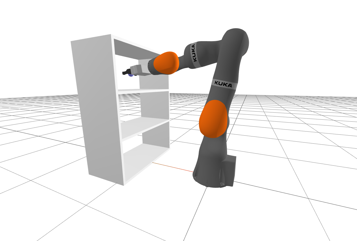
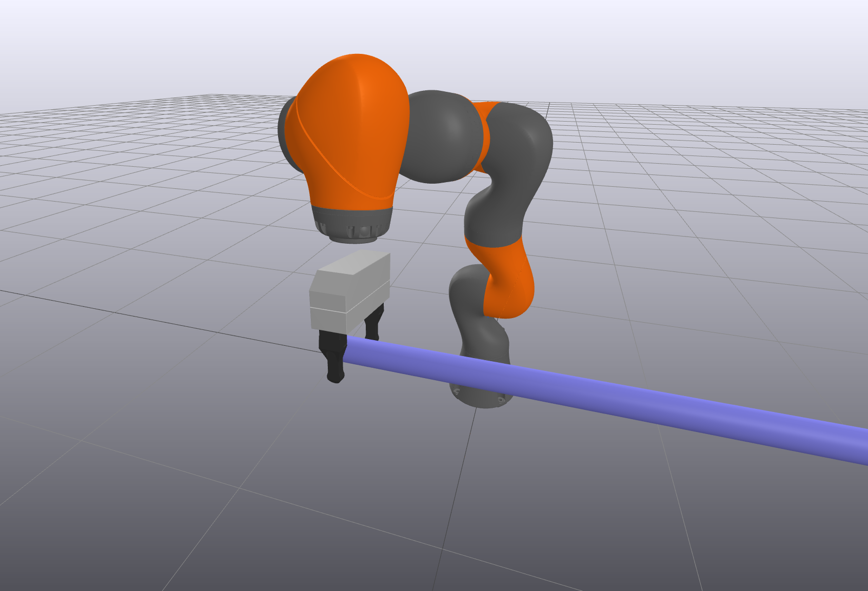
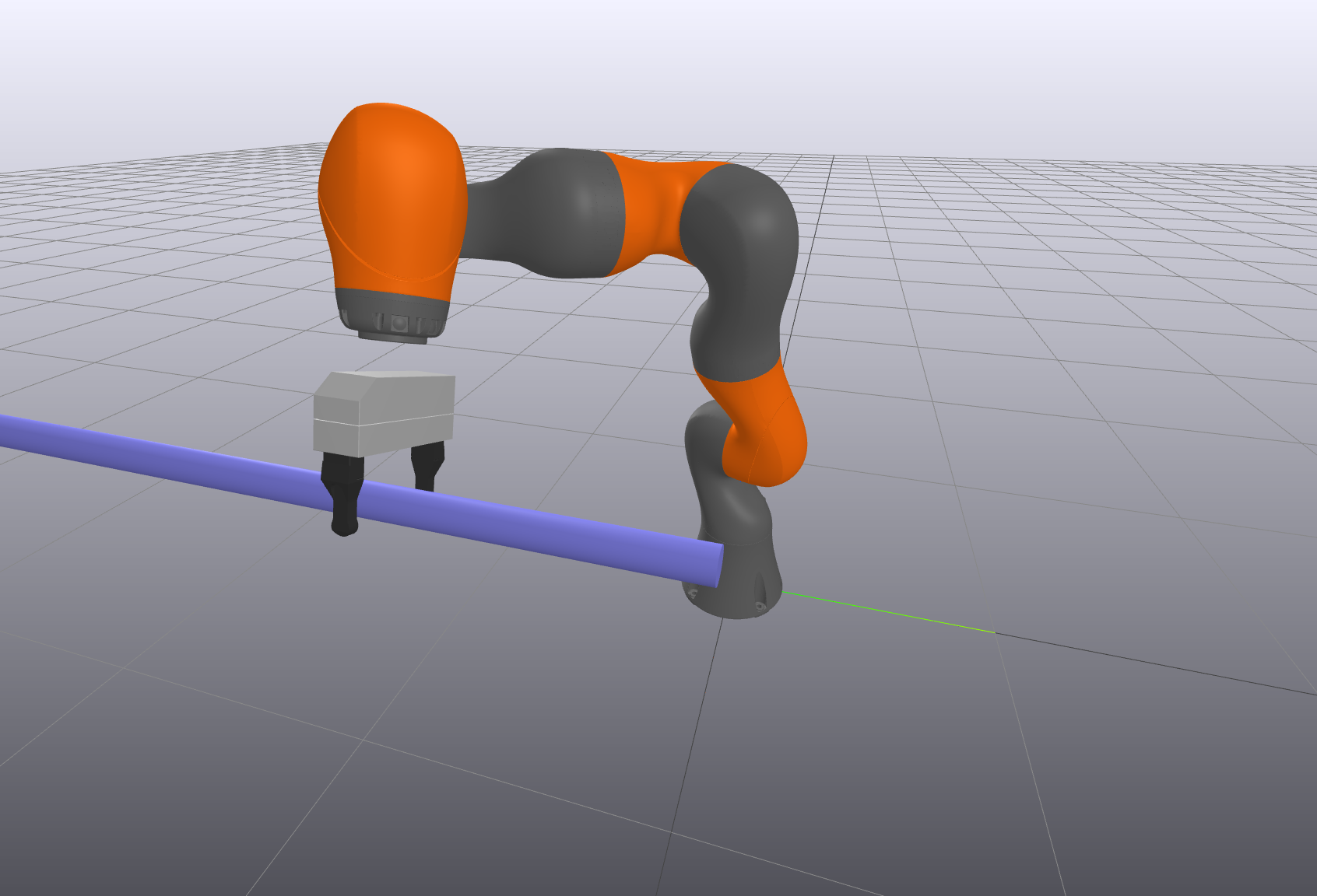
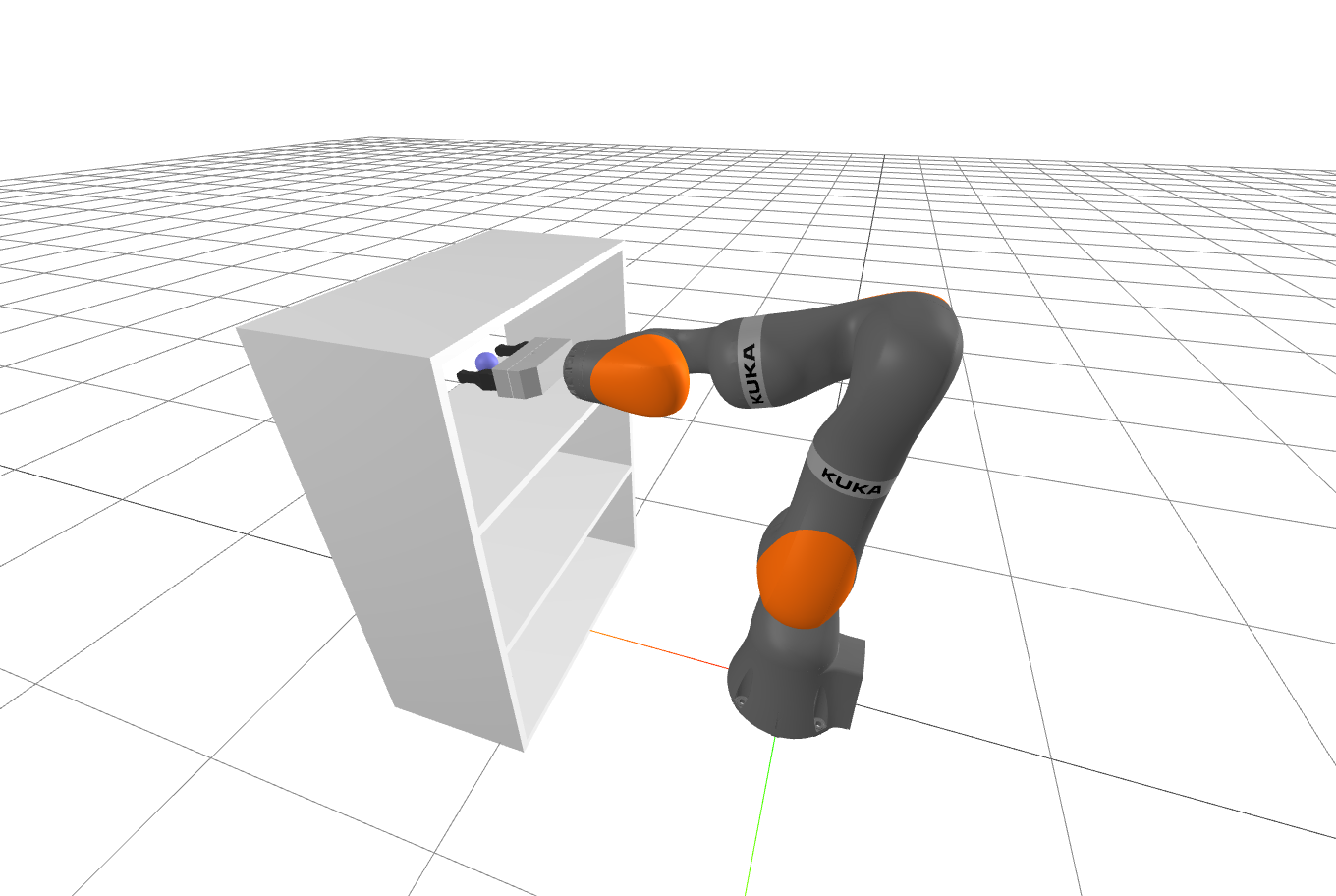
A
richer inverse kinematics problem: solve for the joint angles, $q$, that
allow the robot to reach into the shelf and grab the object, while
avoiding collisions.
We have already
discussed the idea of solving differential inverse kinematics
as an optimization problem. In that workflow, we started by using the
pseudo-inverse of the kinematic Jacobian, but then graduated to thinking
about the least-squares formulation of the inverse problem. The more
general least-squares setting, we could add additional costs and
constraints that would protect us from (nearly) singular Jacobians and
could take into account additional constraints from joint limits, joint
velocity limits, etc. We could even add collision avoidance constraints.
Some of these constraints are quite nonlinear / nonconvex functions of
the configuration $q$, but in the differential kinematics setting we were
only seeking to find a small change $\Delta q$ around the nominal
configuration, so it was quite reasonable to make linear/convex
approximations of these nonlinear/nonconvex constraints.
Now we will consider the full formulation, where we try to solve the
nonlinear / nonconvex optimization directly, without any constraints on
only making a small change to an initial $q$. This is a much harder
problem computationally. Using powerful nonlinear optimization solvers
like SNOPT, we are often able to solve the problems, even at interactive
rates (the example below is quite fun). But there are no guarantees. It
could be that a solution exists even if the solver returns
"infeasible".
Of course, the differential IK problem and the full IK problem are
closely related. In fact, you can think about the differential IK
algorithm as doing one step of (projected) gradient descent or one-step
of Sequential Quadratic Programming,
for the full nonlinear problem.
Drake provides a nice InverseKinematics
class that makes it easy to assemble many of the standard
kinematic/multibody constraints into a
MathematicalProgram. Take a minute to look at the
constraints that are offered. You can add constraints on the relative
position and/or orientation on two bodies, or that two bodies are more
than some minimal distance apart (e.g. for non-penetration) or closer
than some distance, and more. This is the way that I want you to think
about the IK problem; it is an inverse problem, but one with a
potentially very rich set of costs and constraints.
Interactive IK
Despite the nonconvexity of the problem and nontrivial computational
cost of evaluating the constraints, we can often solve it at
interactive rates. I've assembled a few examples of this in the
chapter notebook:
In the first version, I've added sliders to let you control the
desired pose of the end-effector. This is the simple version of the IK
problem, amenable to more explicit solutions, but we nevertheless solve
it with our full nonlinear optimization IK engine (and it does include
joint limit constraints). This demo won't look too different from the
very first example in the notes, where you used teleop to command the
robot to pick up the red brick. In fact, differential IK offers a fine
solution to this problem, too.
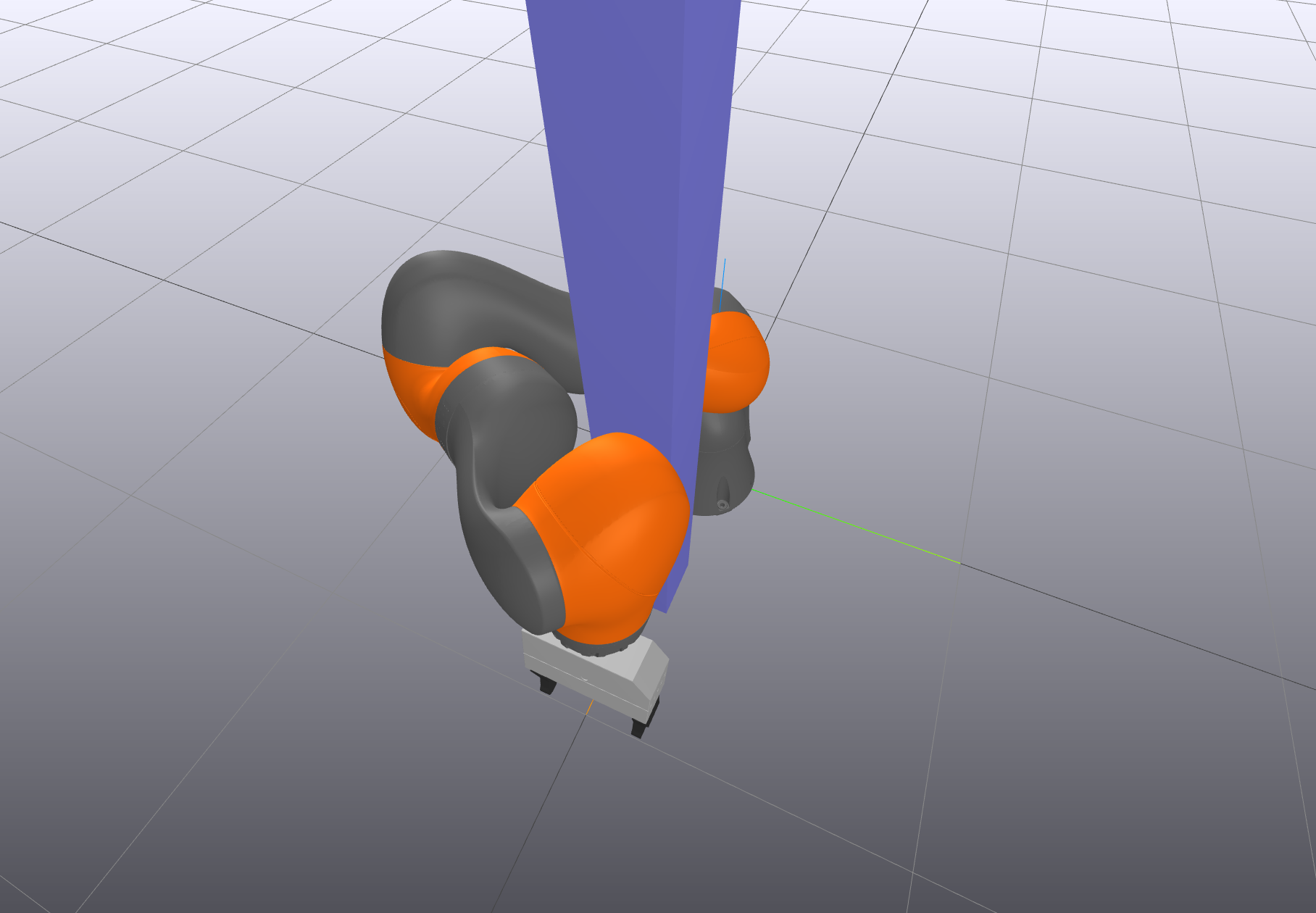
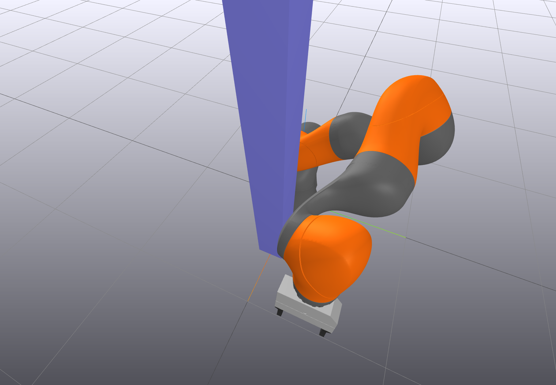
In the second example, I've tried to highlight the differences
between the nonlinear IK problem and the differential IK problem by
adding an obstacle directly in front of the robot. Because both our
differential IK and IK formulations are able to consume the
collision-avoidance constraints, both solutions will try to prevent you
from crashing the arm into the post. But if you move the target
end-effector position from one side of the post to the other, the full
IK solver can switch over to a new solution with the arm on the other
side of the post, but the differential IK will never be able to make
that leap (it will stay on the first side of the post, refusing to
allow a collision).
As the desired end-effector position moves along
positive $y$, the IK solver is able to find a new solution with the
arm wrapped the other way around the post.
With great power comes great responsibility. The inverse kinematics
toolbox allows you to formulate complex optimizations, but your success
with solving them will depend partially on how thoughtful you are about
choosing your costs and constraints. My basic advice is this:
Try to keep the objective (costs) simple; I typically only use the
"joint-centering" quadratic cost on $q$. Putting terms that should be
constraints into the cost as penalties leads to lots of cost-function
tuning, which can be a nasty business.
Write minimal constraints.
You want the set of feasible configurations to be as big as possible.
For instance, if you don't need to fully constrain the orientation of the
gripper, then don't do it.
I'll follow-up with that second
point using the following example.
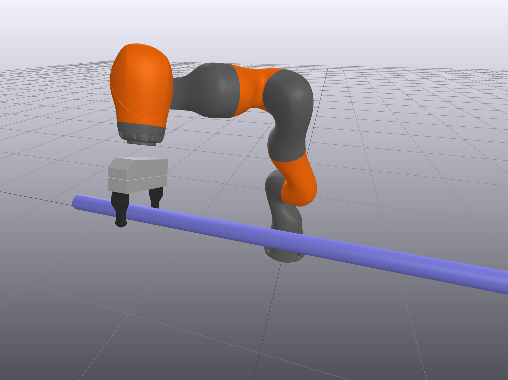
Grasp the cylinder
Let's use IK to grasp a cylinder. You can think of it as a hand
rail, if you prefer. Suppose it doesn't matter where along the
cylinder we grasp, nor the orientation at which we grasp it. Then we
should write the IK problem using only the minimal version of those
constraints.
In the notebook, I've coded up one version of this. I've put the
cylinder's pose on the sliders now, so you can move it around the
workspace, and watch how the IK solver decides to position the robot.
In particular, if you move the cylinder in $\pm y$, you'll see that the
robot doesn't try to follow... until the hand gets to the end of the
cylinder. Very nice!
One could imagine multiple ways to implement that constraint.
Here's how I did it:
In words, I've defined two points in the gripper frame; in the notation
of the AddPositionConstraint method they are ${}^Bp^{Q}$.
Recall the gripper frame is such
that $[0, .1, 0]$ is right between the two gripper pads; you should
take a moment to make sure you understand where $[0,.1,-0.02]$ and
$[0,.1,0.02]$ are. Our constraints require that both of those points
should lie exactly on the center line segment of the cylinder. This
was a compact way for me to leave the orientation around the cylinder
axis as unconstrained, and capture the cylinder position constraints
all quite nicely.
We've provided a rich language of constraints for specifying IK
problems, including many which involve the kinematics of the robot and
the geometry of the robot and the world (e.g., the minimum-distance
constraints). Let's take a moment to appreciate the geometric puzzle
that we are asking the optimizer to solve.
Visualizing the configuration space
Let's return to the example of the iiwa reaching into the shelf.
This IK problem has two major constraints: 1) we want the center of the
target sphere to be in the center of the gripper, and 2) we want the
arm to avoid collisions with the shelves. In order to plot these
constraints, I've frozen three of the joints on the iiwa, leaving only
the three corresponding motion in the $x-z$ plane.
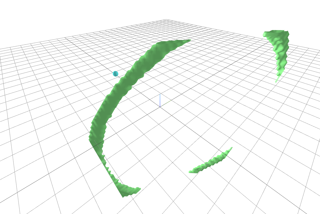
The image on the right is a visualization of the "grasp
the sphere" constraint in configuration space -- the x,y,z, axes in
the visualizer correspond to the three joint angles of the
planarized iiwa.
To visualize the constraints, I've sampled a dense grid in the three
joint angles of the planarized iiwa, assigning each grid element to 1
if the constraint is satisfied or 0 otherwise, then run a marching
cubes algorithm to extract an approximation of the true 3D geometry of
this constraint in the configuration space. The "grasp the sphere"
constraint produces the nice green geometry I've pictured above on the
right; it is clipped by the joint limits. The collision-avoidance
constraint, on the other hand, is quite a bit more complicated. To see
that, you'd better open up this
3D
visualization so you can navigate around it yourself. Scary!
Visualizing the IK optimization problem
To help you appreciate the problem that we've formulated, I've made
a visualization of the optimization landscape. Take a look at the
landscape here first; this
is only plotting a small region around the returned solution. You can
use the Meshcat controls to show/hide each of the individual costs and
constraints, to make sure you understand.
As recommended, I've kept the cost landscape (the green
surface) to be simply the quadratic joint-centering cost. The
constraints are plotted in blue when they are feasible, and
red when they are infeasible:
The joint limit constraint is just a simple "bounding-box"
constraint here (only the red infeasible region is drawn for bounding
box constraints, to avoid making the visualization too
cluttered).
The position constraint has three elements: for the $x$, $y$, and
$z$ positions of the end-effector. The $y$ position constraint is
trivially satisfied (all blue) because the manipulator only has the
joints that move in the $x-z$ plane. The other two look all red, but
if you turn off the $y$ visualization, you can see two small strips
of blue in each. That's the conditions in our tight position
constraint.
But it's the "minimum-distance" (non-collision) constraint that is the most impressive / scary of all. While we visualized the configuration space above, you can see here that visualizing the distance as a real-valued function reveals the optimization landscape that we give to the solver.
The intersection of all the blue regions here are what defined
the configuration-space in the example above. All of the code for this
visualization is available in the notebook, and you can find the exact
formulation of the costs and constraints there:
You should also take a quick look at the full optimization landscape. This
is the same set of curves as in the visualization above, but now it's
plotted over the entire domain of joint angles within the joint limits.
Nonlinear optimizers like SNOPT can be pretty amazing sometimes!
Global inverse kinematics
For unconstrained inverse kinematics with exactly six degrees of
freedom, we have closed-form solutions. For the generalized inverse
kinematics problem with rich costs and constraints, we've got a nonlinear
optimization problem that works well in practice but is subject to local
minima (and therefore can fail to find a feasible solution if it exists).
If we give up on solving the optimization problem at interactive rates,
is there any hope of solving the richer IK formulation robustly? Ideally
to global optimality?
This is actually an extremely relevant question. There are many
applications of inverse kinematics that work offline and don't have any
strict timing requirements. Imagine if you wanted to generate training
data to train a neural network to learn your inverse kinematics; this
would be a perfect application for global IK. Or if you want to do
workspace analysis to see if the robot can reach all of the places it
needs to reach in the workspace that you're designing for it, then you'd
like to use global IK. Some of the motion planning strategies that we'll
study below will also separate their computation into an offline
"building" phase to make the online "query" phase much faster.
In my experience, general-purpose global nonlinear solvers -- for
instance, based on mixed-integer nonlinear programming (MINLP) approaches
or the interval arithmetic used in satisfiability-modulo-theories (SMT)
solvers -- typically don't scale the complexity of a full manipulator.
But if we only slightly restrict the class of costs and constraints that
we support, then we can begin to make progress.
Drake provides an implementation of the GlobalInverseKinematics
approach described in Dai17 using mixed-integer convex
optimization. The solution times are on the order of a few seconds; it
can solve a full constrained bimanual problem in well under a minute.
Trutman22 solves the narrow version of the problem (just
end-effector poses and joint limits) using convex optimization via a
hierarchy of semi-definite programming relaxations; it would be very
interesting to understand how well this approach works with the larger
family of costs and constraints.
Inverse kinematics vs differential inverse kinematics
When should we use IK vs Differential IK? IK solves a more global
problem, but is not guaranteed to succeed. It is also not guaranteed to
make small changes to $q$ as you make small changes in the
cost/constraints; so you might end up sending large $\Delta q$ commands
to your robot. Use IK when you need to solve the more global problem,
and the trajectory optimization algorithms we produce in the next section
are the natural extension to producing actual $q$ trajectories.
Differential IK works extremely well for incremental motions -- for
instance if you are able to design smooth commands in end-effector space
and simply track them in joint space.
Grasp planning using inverse kinematics
In our first version of grasp
selection using sampling, we put an objective that rewarded grasps
that were oriented with the hand grasping from above the object. This was
a (sometimes poor) surrogate for the problem that we really wanted to
solve: we want the grasp to be achievable given a "comfortable" position
of the robot. So a simple and natural extension of our grasp scoring
metric would be to solve an inverse kinematics problem for the grasp
candidate, and instead of putting costs on the end-effector orientation,
we can use the joint-centering cost directly as our objective.
Furthermore, if the IK problem returns infeasible, we should reject the
sample.
There is a quite nice extension of this idea that becomes natural once
we take the optimization view, and it is a nice transition to the
trajectory planning we'll do in the next section. Imagine if the task
requires us not only to pick up the object in clutter, but also to place
the object carefully in clutter as well. In this case, a good grasp
involves a pose for the hand relative to the object that
simultaneously optimizes both the pick configuration and the place
configuration. One can formulate an optimization problem with decision
variables for both $q_{pick}$ and $q_{place}$, with constraints enforcing
that ${}^OX^{G_{pick}} = {}^OX^{G_{place}}$. Of course we can still add
in all of our other rich costs and constraints, In the dish-loading project at TRI, this
approach proved to be very important. Both picking up a mug in the sink
and placing it in the dishwasher rack are highly constrained, so we
needed the simultaneous optimization to find successful grasps.
Simple code example here
Kinematic trajectory optimization
Once you understand the optimization perspective of inverse kinematics, then you
are well on your way to understanding kinematic trajectory optimization. Rather than
solving multiple inverse kinematics problems independently, the basic idea now is to
solve for a sequence of joint angles simultaneously in a single optimization. Even
better, let us define a parameterized joint trajectory, $q_\alpha(t)$, where
$\alpha$ is a vector of parameters. Then a simple extension to our inverse
kinematics problem would be to write something like \begin{align} \min_{\alpha,T} &
\quad T, \\ \subjto &\quad X^{G_{start}} = f_{kin}(q_\alpha(0)),\\ & \quad
X^{G_{goal}} = f_{kin}(q_\alpha(T)), \\ & \quad \forall t , \quad
\left|\dot{q}_\alpha(t)\right| \le v_{max} \label{eq:vel_limits}. \end{align} I read
this as "find a trajectory, $q_\alpha(t)$ for $t \in [0, T]$, that moves the gripper
from the start to the goal in minimum time".
The last equation, (\ref{eq:vel_limits}), represents velocity limits;
this is the only way we are telling the optimizer that the robot cannot
teleport instantaneously from the start to the goal. Apart from this line
which looks a little non-standard, it is almost exactly like solving two
inverse kinematics problems jointly, except instead of having the solver
take gradients with respect to $q$, we will take gradients with respect to
$\alpha$. This is easily accomplished using the chain rule.
Trajectory parameterizations
The interesting question, then, becomes how do we actually
parameterize the trajectory $q(t)$ with a parameter vector $\alpha$?
These days, you might think that $q_\alpha(t)$ could be a neural network
that takes $t$ as an input, offers $q$ as an output, and uses $\alpha$ to
represent the weights and biases of the network. Of course you could, but
for inputs with a scalar input like this, we often take much simpler and
sparser parameterizations, often based on polynomials.
There are many ways one can parameterize a trajectory with
polynomials. For example in dynamic motion planning, direct
collocation methods use piecewise-cubic
polynomials to represent the state trajectory, and the pseudo-spectral
methods use Lagrange polynomials. In each case, the choice of basis
functions is made so that algorithm can leverage a particular property of
the basis. In dynamic motion planning, a great deal of focus is on the integration accuracy of the dynamic equations to ensure that we obtain feasible solutions to the dynamic constraints.
When we are planning the motions of our fully-actuated robot arms, we
typically worry less about dynamic feasibility, and focus instead on the
kinematics. For kinematic trajectory optimization, the so-called
B-spline
trajectory parameterization has a few particularly nice properties
that we can leverage here:
The derivative of a B-spline is still a B-spline (the degree is
reduced by one), with coefficients that are linear in the original
coefficients.
The bases themselves are non-negative and sparse.
This gives the coefficients of the B-spline polynomial, which are
referred to as the control points, a strong geometric
interpretation.
In particular, the entire trajectory is guaranteed to lie inside the
convex hull of the active control points (the control points who's bases
are not zero).
Taken together this means that we can optimize over finitely
parameterized trajectories, but use the convex hull property to ensure
that limits on the joint positions and any of its derivatives are
satisfied $\forall t\in [0,T]$ using linear constraints. This
sort of guarantee would be much more costly to obtain using most other
polynomial bases.
Write up the B-spline math here; and clean up the Drake
notation/implementation in the process. In particular, I want to purge
the use of symbolic from KinematicTrajectoryOptimization. My
`RussTedrake/drake:bsplinebasis_derivatives` branch has a start at
getting analytical derivatives for the trajopt workflow.
Note that B-splines are closely
related to Bézier
curves. But the "B" in "B-spline" actually just stands for "basis"
(no, I'm not kidding) and "Bézier splines"
are slightly different.
A simple interactive gui for moving around the control points and visualizing the spline.
Optimization algorithms
The default KinematicTrajectoryOptimization
class in Drake optimizes a trajectory defined using a B-spline to
represent a path, $r(s)$ over the interval $s \in [0,1]$, plus an
additional scalar decision variable corresponding to the trajectory
duration, $T$. The final trajectory combines the path with the
time-rescaling: $q(t) = r(t/T).$ This is a particularly nice way to
represent a trajectory of unknown duration, and has the excellent feature
that the convex hull property can still be used. Velocity constraints are
still linear; constraints on acceleration and higher derivatives do
become nonlinear, but if satisfied they still imply strict bounds
$\forall t \in [0, T].$
Since the KinematicTrajectoryOptimization is written
using Drake's MathematicalProgram, by default it will
automatically select what we think is the best solver given the available
solvers. If the optimization has only convex costs and constraints, it
will be dispatched to a convex optimization solver. But most often we add
in nonconvex costs
and constraints from kinematics. Therefore in most cases, the default
solver would again be the SQP-solver, SNOPT. You are free to experiment
with others!
One of the most interesting set of constraints that we can add to our
kinematic trajectory optimization problem is the MinimumDistanceLowerBoundConstraint;
when the minimum distance between all potential collision pairs is
greater than zero then we have avoided collisions. Please note, though,
that these collision constraints can only be enforced at discrete
samples, $s_i \in [0,1]$, along the path. They do not guarantee that
the trajectory is collision free $\forall t\in[0,T].$ It required
very special properties of the derivative constraints to leverage the
convex hull property; we do not have them for more general nonlinear
constraints. A common strategy is to add constraints at some modest
number of samples along the interval during optimization, then to check
for collisions more densely on the optimized trajectory before executing
it on the robot.
Kinematic trajectory optimization for moving between shelves
As a warm-up, I've provided a simple example of the planar iiwa
reaching from the top shelf into the middle shelf.
If you look carefully at the code, I actually had to solve this
trajectory optimization twice to get SNOPT to return a good solution
(unfortunately, since it is a local optimization, this can happen). For
this particular problem, the strategy that worked was to solve once
without the collision avoidance constraint, and then use that
trajectory as an initial guess for the problem with the collision
avoidance constraint.
Another thing to notice in the code is the "visualization callback"
that I use to plot a little blue line for the trajectory as the
optimizer is solving. Visualization callbacks are implemented by e.g.
telling the solver about a cost function that depends on all of the
variables, and always returns zero cost; they get called every time the
solver evaluates the cost functions. What I've done here can definitely
slow down the optimization, but it's an excellent way to get some
intuition about when the solver is "struggling" to numerically solve a
problem. I think that the people / papers in this field with the
fastest and most robust solvers are highly correlated with people who
spend time visualizing and massaging the numerics of their solvers.
Kinematic trajectory optimization for clutter clearing
We can use KinematicTrajectoryOptimization to do the
planning for our clutter clearing example, too. This optimization was
more robust, and did not require solving twice. I only seeded it with a
trivial initial trajectory to avoid solutions where the robot tried to
rotate 270 degrees around its base instead of taking the shorter
path.
Show example(s) from TRI dish-loading.
There are a number of related approaches to kinematic trajectory
optimization in the motion planning literature, which differ either by
their parameterization or by the solution technique (or both). Some of
the more well-known include CHOMP
Ratliff09a, STOMP Kalakrishnan11a, and
KOMOToussaint17.
KOMO, for instance, is one of a handful of trajectory optimization
techniques that use the Augmented
Lagrangian method of transcribing a constrained optimization problem
into an unconstrained problem, then using a simple but fast
gradient-based solverToussaint14. Augmented-Lagrangian-based
approaches appear to be the most popular and successful these days; I
hope to provide a nice implementation in Drake soon! But one does have to
be careful in comparing these different solvers -- SNOPT may declare
failure if it cannot optimize the cost and satisfy constraints to the
default tolerances (around 1e-6), while an Augmented-Lagrangian approach
will never report failure and will rarely aim for this level of accuracy.
When kinematic trajectory optimizations succeed, they are an
incredibly satisfying solution to the motion planning problem. They give
a very natural and expressive language for specifying the desired motion
(with needing to sample nonlinear constraints as perhaps the one
exception), and they can be solved fast enough for online planning. The
only problem is: they don't always succeed. Because they are based on
nonconvex optimization, they are susceptible to local minima, and can
fail to find a feasible path even when one exists.
Local minima in collision-free trajectory optimization
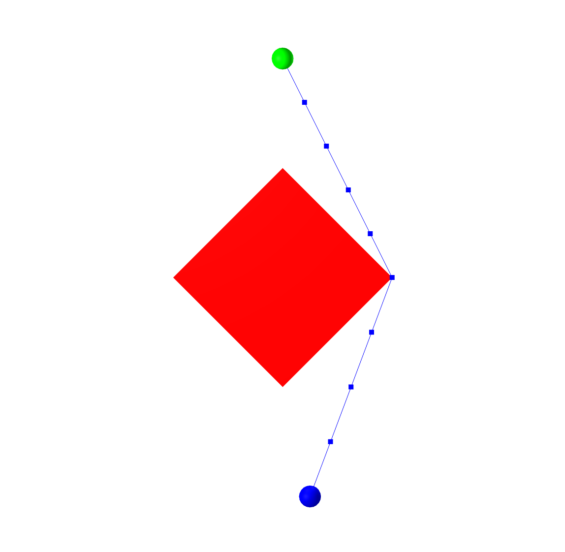
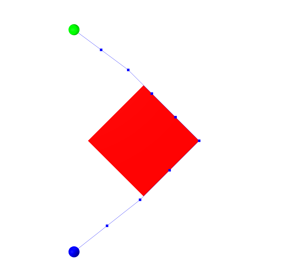
Consider the extremely simple example of finding the shortest path
for a point robot moving from the start (blue circle) to the goal
(green circle) in the image below, avoiding collisions with the red
box. Avoiding even the complexity of B-splines, we can write an
optimization of the form: \begin{aligned} \min_{q_0, ..., q_N} \quad &
\sum_{n=0}^{N-1} | q_{n+1} - q_n|_2^2 & \\ \text{subject to} \quad &
q_0 = q_{start} \\ & q_N = q_{goal} \\ & |q_n|_1 \ge 1 & \forall n,
\end{aligned} where the last line is the collision-avoidance constraint
saying that each sample point has to be outside of the
$\ell_1$-ball (my convenient choice for the geometry of the red box).
Alternatively, we can write a slightly more advanced constraint to
maintain that each line segment is outside of the obstacle
(rather than just the vertices). Here are some possible solutions to this optimization problem:
Fix meshcat line width.
The solution on the left is the (global) minimum for the problem;
the solution on the right is clearly a local minima. Once a nonlinear
solver is considering paths that go right around the obstacle, it is
very unlikely to find a solution that goes left around the obstacle,
because the solution would have to get worse (violate the collision
constraint) before it gets better.
Make a version of this with B-splines
To deal with this limitation, the field of collision-free motion
planning has trended heavily towards sampling-based methods.
Sampling-based motion planning
My aim is to have a complete draft of this section soon! In the mean
time, I strongly recommend the book by Steve LaValleLaValle06,
and checking out the Open Motion
Planning Library. We have strong implementations of the most common
sampling-based algorithms in Drake which are optimized for our
collision engines, and hope to make
them publicly available soon.
Some incredible early (circa 2002) sampling-based motion planning
results from
James Kuffner (hover over the image to animate). These are kinematically complex and quite high dimensional.
There are many optimizations and heuristics which can dramatically
improve the effectiveness of these methods... (optimized collision
checking, weighted Euclidean distances, ...)
Motion Planning w/ Graphs of Convex Sets (GCS)
Trajectory optimization techniques allow for rich specifications of costs and
constraints, including derivative constraints on continuous curves, and can scale to
high-dimensional configuration spaces, but they are fundamentally based on local
(gradient-based) optimization and suffer from local mimima. Sampling-based planners
reason more globally and provide a notion of (probabilistic) completeness, but
struggle to accommodate derivative constraints on continuous curves and struggle in
high dimensions. Is there any way to get the best of both worlds?
My students and I have been working on new approach to motion planning
that attempts to bridge this gap. It builds on a general optimization
framework for mixing continuous optimization and combinatorial optimization
(e.g. on a graph), which we call "Graphs of Convex Sets" (GCS).
To motivate it, let's think about why the PRM struggles to handle
continuous curvature constraints. During the roadmap construction phase, we
do a lot of work with the collision checker to certify that straight line
segments connecting two vertices are collision free (typically only up to
some sampling resolution, though it is possible to do better
Amice23). Then, in the online query phase, we search the discrete graph
to find a (discontinuous) piecewise-linear shortest path from the start to the goal.
Once we go to smooth that path or approximate it with a continuous curve, there is
no guarantee that this path is still collision free, and it certainly might not be
the shortest path. Because our offline roadmap construction only considered line
segments, it didn't leave any room for online optimization. This becomes even more
of a concern when we bring in dynamics -- paths that are kinematically feasible
might not be feasible once we have dynamic constraints. While sampling-based
planning can be
adapted to these so-called "kino-dynamic planning" or "control-based planning"
problems, for a number of subtle reasons these
algorithms have not been as successful as the purely kinematic sampling-based
planning versions.
Add a PRM => GCS plot here.
A relatively small change to the PRM workflow is this: every time we pick a
sample, rather than just adding the configuration-space point to the graph, let's
expand that point into a (convex) region in configuration space. We'll happily pay
some offline computation in order to find nice big regions, because the payoff for
the online query phase is significant. First, we can make much sparser graphs -- a
small number of regions can cover a big portion of configuration space -- which also
allows us to scale to higher dimensions. But perhaps more importantly, now we have
the flexibility to optimize online over continuous curves, so long as they stay
inside the convex regions. This requires a generalization of the graph-search
algorithm which can jointly optimize the discrete path through the graph along with
the parameters of the continuous curves; this is exactly the generalization that GCS
provides.
Graphs of Convex Sets
The GCS framework was originally introduced in
Marcucci21, and we have a mature implementation
in Drake. It is a general optimization framework for combining combinatorial
optimizations, like graph search, with continuous optimizations, like the
kinematic trajectory optimization we studied above. GCS can provide a continuous
extension to any "network flow" optimization (c.f. Ahuja93), but for
motion planning, the first problem we are interested in is shortest paths on a
graph.
Consider the very classical problem of finding the (weighted) shortest
path from a source, $s$, to a target, $t,$ on a graph, pictured on the
left. The problem is described by a set of vertices, a set of
(potentially directed) edges, and the cost of traversing each edge.
GCS provides a simple, but powerful generalization to this problem:
whenever we visit a vertex in the graph, we are also allowed to pick one
element out of a convex set associated with that vertex. Edge lengths are
allowed to be convex functions of the continuous variables in the
corresponding sets, and we can also write convex constraints on the edges
(which must be satisfied by any solution path).
The shortest path problem on a graph of convex sets can encode
problems that are NP-Hard, but these can be formulated as a mixed-integer
convex optimization (MICP). What makes the framework so powerful is that
this MICP has a very strong and efficient convex relaxation;
meaning that if you relax the binary variables to continuous variables
you get (nearly) the solution to the original MICP. This means that you
can solve GCS problems to global optimality orders of magnitude faster
than previous transcriptions. But in practice, we find that solving
only the convex relaxation (plus a little rounding) is almost always
sufficient to recover the optimal solution. Nowadays, we almost never
solve the full MICP in our robotics applications of GCS.
You can find more details and examples about GCS in my underactuated notes,
and a thorough and very readable treatment of GCS as a general tool for
mixed-discrete and continous optimization in Marcucci24a.
GCS (Kinematic) Trajectory Optimization
GCS provides a very general machinery for optimizing over the mixed
discrete/continuous optimization problems that are naturally represented on a
graph. But how do we transcribe the motion planning problem into a GCS? We first
presented the transcription I'll describe here in the paper titled "Motion
planning around obstacles with convex optimization" Marcucci23a. Since
we've already spent time in this chapter talking about the inherent nonconvexity
of the motion planning problem, you can see why we like this title! It should be
slightly surprising that we can use convex optimization to effectively solve these
problems to global optimality.
Let us assume for a moment that we are given a convex decomposition of the
collision-free space. This is a strong assumption, which we will justify below.
Left: A simple 2D configuration-space with obstacles in red.
Right: A convex decomposition of the collision-free configuration space.
Observe that if we have two points in the same convex collision-free region,
then we know that the straight line connecting them is also guaranteed to be
collision free. When points lie in the intersection of two C-space regions, then
they can connect continuous paths through multiple regions. This is the essence of
our transcription. What this implies is that for each visit to a vertex in the
GCS, then we want to pick two points in a C-space region, so that the path
lies in the region. So the convex sets in the GCS are not the C-space regions
themselves, they are the set with $2n$ variables for an $n$-dimensional
configuration space where the first $n$ and the last $n$ are both in the C-space
region. In set notation, we'd say it's the Cartesian product of the set with
itself. We form undirected edges between these sets iff the C-space regions
intersect, and we put a constraint on each edge saying that the second point in
the first set must be equal to the first point in the second set.
GcsTrajOpt in a simple 2D configuration space
Let's run GCS trajectory optimization on the simple configuration space
depicted above. I've put the start in the bottom left corner and the goal in the
top right. I'll run the algorithm twice, once with a minimum-distance objective,
and once with a minimum-time objective (and velocity constraints):
Left: The GcsTrajOpt solution with a minimum-distance cost.
Right: The GcsTrajOpt solution with a minimum-time cost (and velocity constraints).
We can generalize this significantly. Rather than just putting a line
segment in each set, we can use the convex hull property of Bezier curves
to guarantee that an entire continuous path of fixed degree lies inside
the set. Using the derivative properties of the Bezier curves, we can add
convex constraints on the velocities (e.g. velocity limits), and
guarantee that the curves are smooth even at the intersections between
regions. To define these velocities, though, we need to know something
about the rate at which we are traversing the path, so we also introduce
the time-scaling parameterization, much like we did in the kinematic
trajectory optimization above, with time scaling parameters in each
convex set.
The result is a fairly rich trajectory optimization framework that
encodes many (but admittedly not all) of the costs and constraints that
we want for trajectory optimization in the GCS convex optimization
framework. For instance, we can write objectives that include:
time (trajectory duration),
path length (approximated with an upper bound),
an upper bound on path "energy" (e.g. $\int |\dot{q}(t)|_2^2$),
and constraints that include:
path derivative continuity (to arbitrary
degree),
velocity constraints (strictly enforced for all $t$, not just at
sample points),
additional convex position and/or path derivative constraints, such
as initial and final positions and velocities.
We automatically impose path continuity constraints, and the region
constraints (that the entire trajectory stays inside the union of the
C-space regions) which are guaranteed at all $t$, not just at sample points.
You can find the implementation
in Drake here.
GcsTrajOpt in a simple 2D configuration space (cont.)
This is the result of running nearly the same minimum-time optimization as in
the example above, but this time we parameterize each segment with a fifth order
Bezier curve and a time scaling, and ask for continuity up to the fourth
derivative ("snap").
Inspection of the trajectory derivatives reveals that the velocities are
smooth and that they stay within the velocity bounds $[-1, 1]$ for the
entire trajectory; not just at sample points.
Nonconvex trajectory optimization can, of course, consume richer costs and
constraints, but does not have the global optimization and completeness elements
that GCS can provide. We are constantly adding more costs and constraints into
the GCS Trajectory Optimization framework -- some seemingly nonconvex constraints
actually have an exact convex reformulation, others have nice convex
approximations. This leads to a natural merger of the two techniques: we can use
convex approximations of more complex costs and constraints in the GCS convex
relaxation, but then use nonlinear optimization during in the rounding step to
handle the nonconvexity exactly once GCS selects the discrete path through the
graph to give a strong initial guess Wrangel24. This can be
accomplished in Drake via the
use_in_transcription option of the AddCost and AddConstraint methods of
GCS, and adding nonconvex constraints only to the Transcription::kRestriction.
Lots more examples
Convex decomposition of (collision-free) configuration
space
Ok, so how do we obtain a convex decomposition of collision-free configuration
space? Let's start by taking the analogy with the PRM seriously. If we sample a
collision-free point in the configuration space, then what is the right way to
inflate that point into a convex region?
The answer is simpler when we are dealing with convex geometries. In
my view, it is reasonable to approximate the geometry of a robot with
convex shapes in the Euclidean space, $\Re^3.$ Even though many robots
(like the iiwa) have nonconvex mesh geometries, we can often approximate
them nicely as the union of simpler convex geometries; sometimes these
are primitives like cylinders and spheres, alternatively we can perform a
convex decomposition directly on the mesh. But even when the geometries
are convex in the Euclidean space, it is generally unreasonable to
treat them as convex in the configuration space.
There are a few exceptions. If your configuration space only involves
translations, or if your robot geometry is invariant to rotations (e.g. a
point robot or a spherical robot), then the configuration space will
still be convex; this was one of the first key observations that cemented
the notion of configuration space as a core mathematical object in
robotics Lozano-Perez90. This can work for a mobile robot
(even a quadrotor approximated by a sphere). In this case, one can easily
compute the minimum Euclidean distance between any pairs of convex bodies
at the sample point, and for instance, inflate the point into a sphere of
the appropriate radius Shkolnik11a. In order to find bigger
regions, we have made heavy use of the Iterative Region Inflation by
Semidefinite Program (IRIS) algorithm introduced in Deits14
and implemented
in Drake. This algorithm alternates between finding separating
hyperplanes and finding the maximum volume contained ellipse to "inflate"
the region to locally maximize (an efficient approximation of) the volume
of the region.
It is possible to extend the IRIS algorithm to find large convex regions in the more general (nonconvex) configuration space. We've done it in two ways:
Using nonlinear programming (NP). In the IRIS-NP algorithm
Petersen23a (implemented
in Drake), we replace the convex optimization for finding the closest
collision with a nonlinear optimization solver like SNOPT. We randomly sample
potential collisions in order to make the algorithm probabilistically sound; in
practice this algorithm is relatively fast but does not guarantee that
the region is completely collision free. We've recently dramatically improve the
performance of this pipeline with IRIS-NP2,
introduced in Werner24, with creates bigger regions with less faces
orders of magnitude faster than the original IRIS-NP.
Using zero-order optimization (ZO). By replacing the nonlinear
optimization in IRIS-NP with a zeroth-order optimization (no gradients required;
it uses only samples), IRIS-ZO produces slightly smaller regions, but can be
trivially parallelized Werner24.
Using algebraic kinematics + sums-of-squares optimization.
Leveraging the idea that the kinematics of most of our robots can be
expressed using (rational) polynomials, we can use tools from
polynomial optimization to search for rigorous certificates of
non-collision Dai23 (implemented
in Drake). This method tends to be slower, but the results are
sound. The one sacrifice that we have to make here is that we find
convex regions in the stereographic
projection coordinates of the original space. In practice, this represents a slight warping of the coordinate system (and consequently a trajectory length) over the region.
IRIS in Configuration Space
Let's run the IrisInConfigurationSpace (aka IRIS-NP) algorithm
on the example of iiwa reaching into a shelf that we played with before. We will
use the full 7 degrees of freedom of the arm, and the original collision
geometry. I'd like for this example to demonstrate two things: (1) the mechanics
of using IrisInConfigurationSpace and (2) the fact that these IRIS
regions can cover a lot of volume, even when they are up against complicated
configuration-space geometries.
IrisInConfigurationSpace can be configured using a single seed
point; iterations of the algorithm will start with a small region around that
point and "inflate" it to maximize a local approximation of configuration space
volume. We can find a seed configuration, $q,$ that is reaching inside the top
shelf using InverseKinematics. But if we only run IRIS from there,
then the region it will find will not fill space inside the shelf, it will
instead creep out of the shelf in order to cover the much larger configuration
space outside of the shelf. To avoid this, we'll run IRIS twice; once with a
seed that is the "home configuration" of the robot, which will grow a region
outside the shelf. Then we'll run IRIS again with the IK seed inside the shelf,
but with an additional constraint using the first region as an obstacle (asking
that they do not overlap). This will force the second region to use the volume
inside the shelf to maximize volume.
A different approach for obtaining this volume, which I now favor, is to
collect many configuration space samples in the region of interest using inverse
kinematics, then compute the MinimumVolumeCircumscribedEllipsoid
to be used as the starting_ellipse
for IRIS. Then we run only one iteration of IRIS to get a nice region with a
notion of volume corresponding to covering this area of configuration space. This approach avoids the false constraint of using previous regions as obstacles (so leads to bigger regions), runs faster (due to using only one iteration of IRIS), and is more parallelizable.
If we were to continue to follow the analogy with the PRM, then we could
imagine performing a convex decomposition of the space by sampling at random,
rejecting samples that are either in collision or in an existing IRIS region, and
then inflating any remaining samples. But in fact, we can do much better than this
-- we can cover a larger percentage of the configuration free space with the same
number of regions, or alternatively cover a similar volume with less regions. Our
current best algorithm for performing this convex decomposition proceeds by
computing a "minimum clique cover" of the "visibility graph"
Werner23 (implemented in Drake).
GcsTrajOpt in a simple 2D configuration space (cont.)
If we run the "minimum clique cover" algorithm with a coverage threshold of 96% of the configuration space on the simple 2D example, we obtain automatic decompositions like this:
In practice, it seems reasonably tractable to try to compute a quite dense
covering of the configuration space for 7-DOF manipulators, and perhaps even up to
say 10 degrees of freedom. But for higher dimensions, I think that trying to cover
every nook and cranny of the configuration space is a false goal. I strongly
prefer the idea of intializing the clique-cover algorithm with sample points that
represent the "important" regions of your configuration space. Sometimes we do
this by manual seeding (via calls to inverse kinematics), or alternatively, we can
do it by examining trajectories that come from teleop demonstrations, from
another planner (that can generate plans, but without the same guarantees), or
even from a reinforcement learning policy.
The IRIS Builder
Here is a notebook that contains a handful of different tools for steering
the creation of your IRIS regions.
GcsTrajOpt Examples
What's the right cost function for smooth curves?
iiwa reaching into shelves
Bimanual iiwa
Variations and Extensions
Fast path planning (FPP) Marcucci23. Many motion planning
instances don't need the full power of GCS; heuristic approximations can
often find very good solutions. Rather than solving the full GCS problem,
considering the discrete and continuous variables simultaneously, FPP
alternates between solving the discrete and continuous problems to find a
local minima. FPP is (typically) faster than
GcsTrajectoryOptimization, and by virtue of using
alternations, it can handle constraints on the derivatives (e.g.
acceleration constraints) which GcsTrajectoryOptimization
cannot handle. However, FPP is more limited on the class of convex
sets/constraints that it can support. (Drake implementation coming
soon!)
GCS on a manifold including for mobile manipulation
Cohn23, and for bimanual manipulation
Cohn23a.
GCS with dynamic constraints. For discrete-time systems described by
piecewise-affine dynamics and convex objectives and constraints, GCS
provides the strongest formulations to dateMarcucci21. It is
also possible to reason more directly about continuous dynamic
constraints over continuous curves (more coming soon!).
Planning through contact. Amazingly, we now have tight convex
relaxations for quasi-static manipulation with contact
Graesdal24. The initial examples are quite simple (so that
we could study the problem carefully, and defer the details of scaling
the solver), but you can expect much more from us in this direction very
soon.
Planning under uncertainty (coming soon!).
Task and motion planning (coming soon!). Kurtz23 showed a
natural transcription from temporal logic to GCS.
GCS as a (feedback) policy (coming soon!).
Time-optimal path parameterizations
Finish these! Boyd's paper a bit more clear about the writing of the
convex objective. Tobia said he also has some notes on the higher
derivatives.
Once we have a motion plan, a natural question is: what is the fastest
that we can execute that plan, subject to velocity, acceleration, and
torque-limit constraints?
To study this, let's once again define a trajectory $\bq(t)$ defined over
the interval $t \in [t_0, t_f]$ via a path parameterization, ${\bf r}(s)$,
and a time parameterization, $s(t)$, such that $$\bq(t) = {\bf r}(s(t)),
\text{ where }s(t) \in [0,1], s(t_0) = 0, s(t_f) = 1.$$ We will constrain
$\forall t \in [t_0, t_f], \dot{s}(t) > 0,$ so that the inverse mapping
from $s$ to $t$ always exists. The advantage of this parameterization is
that when ${\bf r}(s)$ is fixed, many of the objectives and constraints
that we might want to put on $\bq(t)$ are actually convex in the
derivatives of $s(t).$ To see this, using the shorthand ${\bf r}'(s) =
\pd{\bf r}{s}, {\bf r}''(s) = \pd{^2 {\bf r}}{s^2},$ etc., write
\begin{align*} \dot\bq &= {\bf r}'(s)\dot{s},\\ \ddot\bq(t) &= {\bf r}''(s)
\dot{s}^2 + {\bf r}'(s)\ddot{s}.\end{align*} Even more important/exciting,
substituting these terms into the manipulator
equations yields: $$\bu(s) = {\bf m}(s)\ddot{s} + {\bf c}(s)\dot{s}^2 +
\bar{\bf \tau}_g(s),$$ where $\bu(s)$ is the commanded torque at the scaled
time $s(t)$, and \begin{align} {\bf m}(s) &= {\bf M}({\bf r}(s)){\bf
r}'(s), \\ {\bf c}(s) &= {\bf M}({\bf r}(s)){\bf r}''(s) + \bC({\bf r}(s),
{\bf r}'(s)) {\bf r}'(s), \\ \bar{\bf \tau}_g(s) &= {\bf \tau}_g({\bf
r}(s)).\end{align}
The next key step is to introduce a change of variables: $b(s(t)) =
\dot{s}^2(t) ,$ and note† that $b'(s) = 2 \ddot{s}.$
†
Because $\dot{b}(s) = b'(s)\dot{s}$ and $\dot{b}(s) =
2\dot{s}\ddot{s}.$ We will use a parameterized trajectory to
represent $b(s)$ over the interval $s\in[0,1]$. Let's see that we can write
an extremely useful set of costs and constraints as convex functions of
$b(s)$, evaluated at sampled time points, $s_i = s(t_i)$:
Minimizing the time duration is a convex
objective: $$t_f - t_0 = \int_{t_0}^{t_f} 1 dt = \int_0^1
\frac{1}{\sqrt{b(s)}} ds.$$ This looks nonconvex, but can be written using
...
Although we would like that a finite number of constraints could be
sufficient to imply that these constraints hold over the entire time
interval, $[t_0, t_f]$, in practice, we just enforce the constraints at a
sufficiently large number of sampled times and forgo the strict guarantees.
These time-optimal path parameterizations (TOPP) were studied
extensively throughout the 1980's (e.g. Bobrow85) with bespoke
algorithms that, for instance, attempted to uncover all of the switching
times of the bang-bang trajectory.
Verscheure09+Debrouwere13+Lipp14
made the connections to convex optimization that I've described here.
Pham18 made a popular numerical implementation of this called
TOPPRA
(time-optimal path parameterizations based on reachability analysis). We
make heavy use of these ideas (and spell out the detailed
connections to the Bezier curve parameterization) in
Marcucci23a. You can find a PathParameterizedTrajectory
class in Drake.
One common question is whether TOPP can be used to write convex
constraints on the jerk (or higher derivatives) of the trajectory,
$$\dddot\bq(t) = {\bf r}'''(s) \dot{s}^3(t) + 3{\bf r}''(s) \dot{s}(t)
\ddot{s}(t) + {\bf r}'(s)\dddot{s}(t).$$ This comes up because many
industrial robot manipulators have jerk limits that must be respected.
Debrouwere13
addressed a version of this question. (More soon...)
Exercises
Door Opening
For this exercise, you will implement a optimization-based inverse kinematics solver to open a cupboard door. You will work exclusively in . You will be asked to complete the following steps:
Write down the constraints on the IK problem of grabbing a cupboard handle.
Formalize the IK problem as an instance of optimization.
Implement the optimization problem using MathematicalProgram.
RRT Motion Planning
For this exercise, you will implement and analyze the RRT algorithm introduced in class. You will work exclusively in . You will be asked to complete the following steps:
Implement the RRT algorithm for the Kuka arm.
Answer questions regarding its properties.
Implement the RRT-Connect algorithm for the Kuka arm.
Improving RRT Path Quality
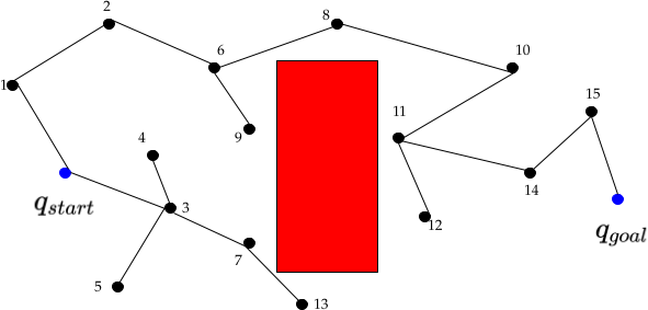
Due to the random process by which nodes are generated, the paths output by RRT can often look somewhat jerky (the "RRT dance" is the favorite dance move of many roboticists). There are many strategies to improve the quality of the paths and in this question we'll explore two. For the sake of this problem, we'll assume path quality refers to path length, i.e. that the goal is to find the shortest possible path, where distance is measured as Euclidean distance in joint space.
One strategy to improve path quality is to post-process paths via "shortcutting", which tries to replace existing portions of a path with shorter segments Geraerts04. This is often implemented with the following algorithm: 1) Randomly select two non-consecutive nodes along the path. 2) Try to connect them with a RRT's extend operator. 3) If the resulting path is better, replace the existing path with the new, better path. Steps 1-3 are repeated until a termination condition (often a finite number of steps or time). For this problem, we can assume that the extend operator is a straight line in joint space. Consider the graph below, where RRT has found a rather jerky path from $q_{start}$ to $q_{goal}$. There is an obstacle (shown in red) and $q_{start}$ and $q_{goal}$ are highlighted in blue (disclaimer: This graph was manually generated to serve as an illustrative example).
Name one pair of nodes for which the shortcutting algorithm would result in a shorter path (i.e. two nodes along our current solution path for which we could produce a shorter path if we were to directly connect them). You should assume the distance metric is the 2D Euclidean distance.
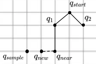
Shortcutting as a post-processing technique, reasons over the existing path and enables local "re-wiring" of the graph. It is a heuristic and does not, however, guarantee that the tree will encode the shortest path. To explore this, let's zoom in one one iteration of RRT (as illustrated below), where $q_{sample}$ is the randomly generated configuration, $q_{near}$ was the closest node on the existing tree and $q_{new}$ is the RRT extension step from $q_{near}$ in the direction of q_sample. When the standard RRT algorithm (which you implemented in a previous exercise) adds $q_{new}$ to the tree, what node is its parent? If we wanted our tree to encode the shortest path from the starting node, $q_{start}$, to each node in the tree, what node should be the parent node of $q_{new}$?
This idea of dynamically "rewiring" to discover the minimum cost path (which for us is the shortest distance) is a critical aspect of the asymptotically optimal variant of RRT known as RRT* Karaman11. As the number of samples tends towards infinity RRT* finds the optimal path to the goal! This is unlike "plain" RRT, which is provably suboptimal (the intuition for this proof is that RRT "traps" itself because it cannot find better paths as it searches).
Decomposing Obstacle-Free Space with Convex Optimization
For this exercise, you will implement part of the IRIS algorithm Deits14, which is used to compute large regions of obstacle-free space through a series of convex optimizations. These regions can be used by various planning methods that search for trajectories from start to goal while remaining collision-free. You will work exclusively in . You will be asked to complete the following steps:
Implement a QP that finds the closest point on an obstacle to an ellipse in free-space.
Implement the part of the algorithm that searches for a set of hyperplanes that separate a free-space ellipse from all the obstacles.
Plan and Place
For this exercise, you will build on the manipulating letter assets exercises from previous chapters. You will use RRT-Connect to plan and simulate a collision-free trajectory for manipulating your initial in a cluttered environment. Then, you will implement shortcutting to improve your path quality and reduce some of the "RRT Dance". You will work exclusively in . You will be asked to complete the following steps:
Define keyframe poses.
Implement an optimization-based inverse kinematics function that, for each keyframe pose, solves for a feasible robot configuration
Implement RRT-Connect.
Implement shortcutting.
Iiwa Path Planning through Shelves Using IRIS and GCS in Joint Space
For this exercise, you will practice finding large collision-free configuration-space regions with IRIS and planning a trajectory through them in joint space with GCS for the Kuka Iiwa manipulator. You will work in . You will be asked to complete the following steps:
Define and compute IRIS regions in joint space around your desired start and end points.
Formulate a GCS trajectory planning problem through your IRIS regions and solve it to plan Iiwa's joint space path.
Trajectory Optimization Around a Shelf Exterior
Through this exercise, you will better understand how the environment around the robot affects the techniques you use when formulating and solving your trajectory optimization problem. Specifically, we'll look at the effects of operating at the boundaries of the Iiwa's kinematic workspace and with complex collision constraints as you move the gripper around the outside of a shelf. You will work in . You will be asked to complete the following steps:
Define and solve a kinematic trajectory optimization in the Kuka Iiwa's full joint space without collision constraints.
Add collision constraints to the prior formulation, use the prior "karate chop" trajectory as an initial guess, and diagnose why this second iteration fails to converge within the default solver parameters.
Investigate how a more informative initial guess will enable faster convergence to a solution.
References
Maurice Fallon and Scott Kuindersma and Sisir Karumanchi and Matthew Antone and Toby Schneider and Hongkai Dai and Claudia Pérez D'Arpino and Robin Deits and Matt DiCicco and Dehann Fourie and Twan Koolen and Pat Marion and Michael Posa and Andrés Valenzuela and Kuan-Ting Yu and Julie Shah and Karl Iagnemma and Russ Tedrake and Seth Teller,
"An Architecture for Online Affordance-based Perception and Whole-body Planning",
Journal of Field Robotics, vol. 32, no. 2, pp. 229-254, September, 2014.
[ link ]
Pat Marion and Maurice Fallon and Robin Deits and Andrés Valenzuela and Claudia Pérez D'Arpino and Greg Izatt and Lucas Manuelli and Matt Antone and Hongkai Dai and Twan Koolen and John Carter and Scott Kuindersma and Russ Tedrake,
"Director: A User Interface Designed for Robot Operation With Shared Autonomy",
Journal of Field Robotics, vol. 1556-4967, 2016.
[ link ]
Charles W. Wampler and Andrew J. Sommese,
"Numerical algebraic geometry and algebraic kinematics",
Acta Numerica, vol. 20, pp. 469-567, 2011.
Rosen Diankov,
"Automated Construction of Robotic Manipulation Programs",
PhD thesis, Carnegie Mellon University, August, 2010.
Hongkai Dai and Gregory Izatt and Russ Tedrake,
"Global inverse kinematics via mixed-integer convex optimization",
International Symposium on Robotics Research, 2017.
[ link ]
Pavel Trutman and Mohab Safey El Din and Didier Henrion and Tomas Pajdla,
"Globally optimal solution to inverse kinematics of 7DOF serial manipulator",
IEEE Robotics and Automation Letters, vol. 7, no. 3, pp. 6012--6019, 2022.
Nathan Ratliff and Matthew Zucker and J. Andrew (Drew) Bagnell and Siddhartha Srinivasa,
"CHOMP: Gradient Optimization Techniques for Efficient Motion Planning",
IEEE International Conference on Robotics and Automation (ICRA) , May, 2009.
Mrinal Kalakrishnan and Sachin Chitta and Evangelos Theodorou and Peter Pastor and Stefan Schaal,
"STOMP: Stochastic trajectory optimization for motion planning",
2011 IEEE international conference on robotics and automation , pp. 4569--4574, 2011.
Marc Toussaint,
"A tutorial on Newton methods for constrained trajectory optimization and relations to SLAM, Gaussian Process smoothing, optimal control, and probabilistic inference",
Geometric and numerical foundations of movements, pp. 361--392, 2017.
Marc Toussaint,
"A Novel Augmented Lagrangian Approach for Inequalities and Convergent Any-Time Non-Central Updates",
, 2014.
Steven M. LaValle,
"Planning Algorithms", Cambridge University Press
, 2006.
Amice and Alexandre and Werner and Peter and Tedrake and Russ,
"Certifying Bimanual RRT Motion Plans in a Second",
International Conference on Robotics and Automation, pp. 9293-9299, 2024.
[ link ]
Tobia Marcucci and Jack Umenberger and Pablo A. Parrilo and Russ Tedrake,
"Shortest Paths in Graphs of Convex Sets",
arxiv, 2023.
[ link ]
Ravindra K Ahuja and Thomas L Magnanti and James B Orlin,
"Network flows: theory, algorithms, and applications", Prentice-Hall, Inc.
, 1993.
Tobia Marcucci,
"Graphs of Convex Sets with Applications to Optimal Control and Motion Planning",
PhD thesis, Massachusetts Institute of Technology, May, 2024.
[ link ]
Tobia Marcucci and Mark Petersen and David von Wrangel and Russ Tedrake,
"Motion planning around obstacles with convex optimization",
Science Robotics, vol. 8, no. 84, 2023.
David von Wrangel and Russ Tedrake,
"Using Graphs of Convex Sets to Guide Nonconvex Trajectory Optimization",
Proceedings of the IEEE/RSJ International Conference on Intelligent Robots and Systems (IROS) , pp. 8, 2024.
[ link ]
Tomas Lozano-Perez,
"Spatial planning: A configuration space approach", Springer
, 1990.
Alexander Shkolnik and Russ Tedrake,
"Sample-Based Planning with Volumes in Configuration Space",
arXiv:1109.3145v1 [cs.RO], 2011.
Robin L H Deits and Russ Tedrake,
"Computing Large Convex Regions of Obstacle-Free Space through Semidefinite Programming",
Proceedings of the Eleventh International Workshop on the Algorithmic Foundations of Robotics (WAFR 2014) , 2014.
[ link ]
Mark Petersen and Russ Tedrake,
"Growing convex collision-free regions in configuration space using nonlinear programming",
arXiv preprint arXiv:2303.14737, 2023.
Peter Werner and Thomas Cohn and Rebecca H. Jiang and Tim Seyde and Max Simchowitz and Russ Tedrake and Daniela Rus,
"Faster Algorithms for Growing Collision-Free Convex Polytopes in Robot Configuration Space",
Accepted to ISRR 2024 , 2024.
[ link ]
Hongkai Dai* and Alexandre Amice* and Peter Werner and Annan Zhang and Russ Tedrake,
"Certified Polyhedral Decompositions of Collision-Free Configuration Space",
The International Journal of Robotics Research (IJRR), vol. 43, no. 9, pp. 1322-1341, November, 2023.
[ link ]
Peter Werner and Alexandre Amice and Tobia Marcucci and Daniela Rus and Russ Tedrake,
"Approximating Robot Configuration Spaces with few Convex Sets using Clique Covers of Visibility Graphs",
International Conference on Robotics and Automation, pp. 10359-10365, 2024.
[ link ]
Tobia Marcucci and Parth Nobel and Russ Tedrake and Stephen Boyd,
"Fast Path Planning Through Large Collections of Safe Boxes",
arXiv preprint arXiv:2305.01072, 2023.
Thomas Cohn and Mark Petersen and Max Simchowitz and Russ Tedrake,
"Non-Euclidean Motion Planning with Graphs of Geodesically-Convex Sets",
Robotics: Science and Systems , 2023.
[ link ]
Thomas Cohn and Seiji Shaw and Max Simchowitz and Russ Tedrake,
"Constrained Bimanual Planning with Analytic Inverse Kinematics",
arXiv preprint arXiv:2309.08770, May, 2024.
[ link ]
Bernhard P Graesdal and Shao Yuan Chew Chia and Tobia Marcucci and Savva Morozov and Alexandre Amice and Pablo A Parrilo and Russ Tedrake,
"Towards Tight Convex Relaxations for Contact-Rich Manipulation",
arXiv preprint arXiv:2402.10312, 2024.
Vince Kurtz and Hai Lin,
"Temporal Logic Motion Planning with Convex Optimization via Graphs of Convex Sets",
arXiv preprint arXiv:2301.07773, 2023.
J.E. Bobrow and S. Dubowsky and J.S. Gibson,
"Time-Optimal Control of Robotic Manipulators Along Specified Paths",
Int. J of Robotics Research, vol. 4, no. 3, pp. 3--17, 1985.
Diederik Verscheure and Bram Demeulenaere and Jan Swevers and Joris De Schutter and Moritz Diehl,
"Time-optimal path tracking for robots: A convex optimization approach",
Automatic Control, IEEE Transactions on, vol. 54, no. 10, pp. 2318--2327, 2009.
Frederik Debrouwere and Wannes Van Loock and Goele Pipeleers and Quoc Tran Dinh and Moritz Diehl and Joris De Schutter and Jan Swevers,
"Time-optimal path following for robots with convex--concave constraints using sequential convex programming",
IEEE Transactions on Robotics, vol. 29, no. 6, pp. 1485--1495, 2013.
Thomas Lipp and Stephen Boyd,
"Minimum-time speed optimisation over a fixed path",
International Journal of Control, vol. 87, no. 6, pp. 1297--1311, 2014.
Hung Pham and Quang-Cuong Pham,
"A new approach to time-optimal path parameterization based on reachability analysis",
IEEE Transactions on Robotics, vol. 34, no. 3, pp. 645--659, 2018.
R. Geraerts and M. Overmars,
"A comparative study of probabilistic roadmap planners",
Algorithmic Foundations of Robotics V, pp. 43--58, 2004.
S. Karaman and E. Frazzoli,
"Sampling-based Algorithms for Optimal Motion Planning",
Int. Journal of Robotics Research, vol. 30, pp. 846--894, June, 2011.